Distributions and Hypothesis Testing
Overview

Click for Full PDF
We have spent the last few weeks working with MySQL and APIs with the goal of helping you understand how data is organized, stored, and accessed. This week, we are going to work within Python to explore our data in more detail.
SciPy
We will introduce a new package this week: SciPy. SciPy extends the capabilities of NumPy, and it is particularly useful for solving advanced mathematical and statistical problems. How Is It Used?
During the week, we will:
enhance our understanding of data and how it is distributed by studying descriptive statistics
explore the normal distribution and why it is such an important concept in data science
differentiate between hypothesis tests and perform the appropriate test for the problem
Introduction to Probability Distributions

Click image for full page PDF
Learning Objectives:
By the end of this module, students will be able to:
Identify discrete vs continuous distributions.
Explain how histograms of raw counts can be converted to probabilities. (Probability Mass Functions or PMF)
Explain how we can calculate a continuous line of probability from a histogram (Kernel Density Estimate)
The big picture:
Ultimately this lesson will help us to transition from viewing a distribution in terms of how often a value has occurred to the likelihood that a value would occur in the future.
Understanding the distribution of our data will also help us decide which statistical tests and which machine learning models are appropriate and which are not. In general, statistical tests are broken into two main groups: parametric tests and non-parametric tests. Parametric tests, when possible, are preferable because they are more powerful and easier to interpret. In order to use parametric tests, the key requirement is that the data follows a normal distribution.
The next few lessons will explore the distribution of your data and will provide you with the tools to effectively describe the distribution. Ultimately, this will allow you to choose the appropriate statistical tests and machine learning models for your data.
Probability Mass Function
The histogram above plots the actual count of values that fall into each bin/bar.
By dividing the raw counts by the overall number of values (n), we can convert the raw counts per bin into the probability that a value will fall into that bin.
A probability can easily be converted into a percentage by multiplying the probability by 100. For example, a probability of 0.10 is the same as 10%.
You can achieve this by adding stat = "density" when you make the histogram. This is a visual representation of the Probability Mass Function (PMF) for Outlet_Establishment_Year.
Discrete Vs Continuous Distributions
A distribution shows what values occur and how frequently those values occurred for a single variable.
Distributions can be classified as being "discrete" or "continuous".
"Discrete": distributions can only take on certain values. Note that discrete values do not have to be integers. A few examples are:
years
the number of children
shoe sizes (10, 10.5, 11, 11.5, 12)
"Continuous": distributions that can take on a nearly infinite number of values. A few examples are:
sales
human height/weight
We can identify discrete vs continuous visually using scatterplots and histograms.
Discrete Distributions
"Outlet establishment year" is a discrete feature. In this case, the values may only be whole numbers. Below is a scatterplot and a histogram involving this feature.
From Discrete PMF to Continuous Kernal Density Estimates (KDE)
In order for us to get estimated probabilities for new values that were not in the original PMF, we can convert our PMF's bars into a continuous line by converting our discrete probability mass to a continuous probability density.
We can estimate the continuous probabilities by transforming our discrete PMF bars into a smoothed curve known as a Kernal Density Estimate.
This estimated probability curve is called a kernel-density estimate (KDE). Basically, a KDE is a way to interpolate between histogram bars so that we can get probability estimates for any value in and around our original distribution.
Describing a Distribution: Measure of Central Tendency

Click for Full PDF
Learning Objectives:
Define three “Measures of Central Tendency” (mean, median, and mode)
Describe the measures of central tendency for a normal distribution
Describe measures of central tendency for positively and negatively skewed distributions
There are two fundamental properties of a distribution that should be included in any description of the data.
Central tendency (what is considered a typical value, or the "center" of the data)
Dispersion (how spread out the data is)
This lesson will explore central tendency, and the next lesson will take a deeper dive into dispersion.
What are Measures of Central Tendency?
A measure of central tendency is a single value that attempts to describe a set of data by identifying the central position within that set of data. In statistics, several different measurements are used to describe the “center” of data. These are mean, median, and mode. Using these three main measures, it is possible to find the central or typical value for a set of data. We can also also apply these measures to find the mean, median, and mode of a probability distribution.
Describing a Distribution: Measure of Dispersion

Click image for full page PDF
Recall from the previous lesson that there are two fundamental properties of a distribution that should be included in any description of the data.
Central tendency (what is considered a typical value, or the "center" of the data)
Dispersion (how spread out the data is)
Learning Objectives:
Use quantitative measures of dispersion to describe the distribution of data
Explain the relationship between variance, standard deviation, and z-scores
Calculate kurtosis
Summary:
This lesson introduced quantitative measures of dispersion to describe how spread out a distribution is. Variance, standard deviation, and z-scores each build upon one another. All values are ultimately based on how far away the data points are from the mean. The farther away the data points are (on average), the greater the dispersion. The units of variance are squared units of the data itself. The standard deviation has the same units as the data. Z-scores are in the units of standard deviations.
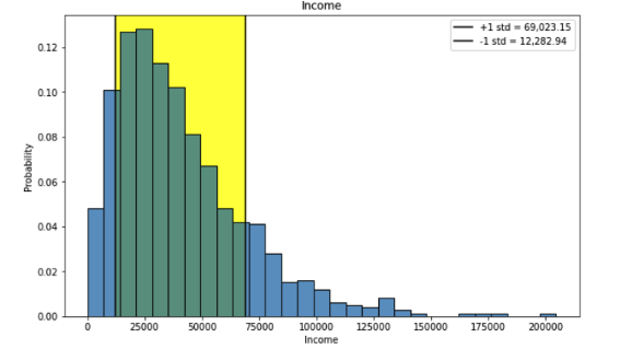
Annotating Distribution Plots
In the lesson exploring measures of central tendency, we provided visuals that showed where the mean, median, or mode occur on the graph. This lesson shows how to add these lines to your visuals.
Learning Objectives:
Add vertical lines to a distribution graph
Highlight a range on a distribution graph
We will use the medical data set for our example:
Summary
This lesson walked through an example of how to add a vertical line to represent the mean to your probability distribution visual. The process is similar for adding a line to represent any value you would like to draw attention to in your visual! Note, that creating visuals is usually an iterative process where you continue to make changes until you are satisfied with the final result! You might want to make further changes to the line style or even the overall style of the graph. You can continue to explore! You can also make more easily reproducible code by defining a variable at the beginning that will be easy to change without having to make as many changes in your existing code. When experimenting with new code, it is a good idea to go step by step so you know what is going on, and then you can put it all together for efficiency!
Click for Full PDF
Standard Normal Distribution
Learning Objectives
Define normal distribution
Define Z-scores / the standard normal distribution
Explain how normal distribution matters within the fields of statistics and Data Science
In the past few lessons, we have been studying distributions and learning how to describe them through both terminology and calculations. A key focus has been determining if a distribution is normal, or in what ways it may deviate from a normal distribution.
What Is Normal Distribution?
The normal distribution is a symmetrical probability distribution with the mean (average) at the center. It is without skew. Data closest to the average occurs more frequently/is more probable than data farthest from the average. In graph form, the normal distribution will appear as a bell-shaped curve. In a normal distribution, the mean, median, and mode are equal.
Properties of the Standard Normal Distribution
Once we have a standard normal distribution, we know exactly what percentage of the data should fall within a specific region of our distribution.
For a normal distribution:
34.1% of the distribution will fall between the mean and 1 standard deviation above the mean and 34.1% will fall 1 standard deviation below the mean.
This means that 68.2% of the distribution falls within mean +/- 1 std (z-score between -1 and 1)
We also know 13.6 % of the distribution falls between +1 std and +2 std and between -1 std and -2 std
This means that 95.4% of the distribution falls within 2 standard deviations (z score between -2 and 2)
An important fact to remember:
Only 2.3% of the distribution falls above and only 2.3% of the distribution falls below 2 standard deviations.
This fact will become very important when we discuss sampling and p-values.
Standard Normal Distribution / Z-Scores
Z scores are sometimes called "standard scores."The z score transformation is especially useful when seeking to compare the relative standings of items from distributions with different means and/or different standard deviations. Z scores are especially informative when the distribution to which they refer is normal. In every normal distribution, the distance between the mean and a given Z score cuts off a fixed proportion of the total area under the curve.
After we convert a normal distribution to z-scores, we refer to it as the standard normal distribution.
Summary
The normal distribution is the most commonly used distribution in statistics. It can be used to determine the proportion of data values that fall within a specified number of standard deviations from the mean. Data science revolves around the concepts of probability distributions, and the core of this concept is focused on Normal Distribution. When the x-axis is z-scores, we consider this the "standard normal distribution," which makes understanding how likely a value is independent of the feature's units. Now that we have concluded the lesson, it is worth revisiting this visual:
When we use the standard normal distribution, we know what percentage of our data is associated with z-score ranges.
Using the Normal Distribution’s PDF/CDF

Click for Full PDF
Lesson Objective:
Differentiate between a pdf and a cdf
Calculate probabilities using the cumulative distribution function.
Using the Normal Distribution's PDF/CDF
Previously, we discussed some properties of the standard normal distribution, including the known % distribution at particular points in the distribution.
When we are working with a normal distribution, we can determine the probability of observing a value within a specific range of values.
We can do this by taking the area under the PDF curve between the 2 values of interest.
Summary
This lesson introduced a cumulative distribution function and showed how it is derived from a probability distribution function. When working with normally distributed data, we showed how using cdf allows us to calculate the probability of any range of values in our distribution.
Defining Hypotheses

Click for full page PDF
Learning Objectives:
Define a Null Hypothesis and an Alternate Hypothesis
Give examples of each
Before performing a statistical test, we need to define what we are testing. There is a formal method for defining our test that involves writing two opposing statements that represent the two possible outcomes of our test. These are known as the null and alternate hypotheses. We will explore these terms with an example.
Null and Alternate Hypotheses
Scenario: A new medicine is being developed for high blood pressure, and its effects on a patient's health are being tested in a clinical trial. There are lots of considerations for designing a clinical test (which can be very interesting!) , but we are focused on understanding how we might define the null and alternate hypothesis. Assume a test group of patients are given the new medicine, while others (in a control group) are given a placebo.
Summary
A first step in performing a statistical test is to write two clear statements that represent the two possible outcomes of your test. These statements are always paired and are always opposite of each other. The null hypothesis states that there is no difference, while the alternate hypothesis states there is a difference. After performing the test, you will either either:
reject the null hypothesis (this means you supported your alternate hypothesis)
accept ("fail to reject") the null hypothesis (this means you did NOT support your alternate hypothesis)
In the next lesson, we will explore how we determine whether we accept or reject our null hypothesis.
P-values and alpha
Learning Objective:
Revisit type 1 and 2 errors in terms of the null and alternate hypotheses
Define p-values and confidence intervals
Determine/interpret if a p-value is significant based on alpha
In the previous lesson, we formally defined our test in terms of the null and alternate hypotheses. When looking for a "difference", we refer specifically to a "statistical difference." This lesson equips you to understand what this means and how it is determined.
One important task of data scientists is to determine if outcomes are meaningful or just due to chance. We use the term "statistical significance" to indicate we have done a statistical test to mathematically determine our results are not just random.
In statistics, we do not work with absolute certainty. Thus, we need to consider the risks of making an error and drawing the incorrect conclusions from our testing. You have encountered these terms previously, but here we will define them in terms of statistical testing:

Click image for full page PDF
Type 1 Error - You erroneously reject the null hypothesis when it is true.
(You support the alternative hypothesis, when it is not true.)
Let's say the new medicine actually has no effect. If your test wrongly concludes that it has made a significant difference, this is a Type 1 Error.
Let's say the individual is actually a human (not an alien), but you wrongly conclude that they must be an alien. This is a Type 1 Error.
Type 2 Error- You erroneously fail to reject the null hypothesis when it is not true. (You do not support the alternative hypothesis when it is true.)
Let's say the new medicine does actually work. You wrongly conclude it made no difference. This is at Type 2 Error.
Let's say the individual actually is an alien, but you wrongly conclude that they are human. This is a Type 2 Error.
For any test, you must consider whether a Type 1 or Type 2 Error is more problematic. Knowing this will help you define the "significance value" or "alpha level" of your test.
Normality Test

Click image for full page PDF
Learning Objectives:
Perform tests for normality
Gain confidence interpreting p-values
A great example of when you might need to interpret p-values occurs when performing a normality test. You do not have to know the mathematics behind the test, but you do need to know how to interpret the results.
Summary
This lesson provides a practical tool for testing normality and a useful example to practice interpreting p-values. You can use the normality test in your data exploration to support your visual analysis. The normality test is just one case where you will need to know how to interpret p-values. Remember, it is essential to know how the null hypothesis is defined to be able to interpret what the results mean for your data. 0.05 is the most common cutoff for determining significance (alpha).
If alpha = 0.05,
A p-value less than 0.05 means reject null hypothesis (accept alternative hypothesis).
A p-value greater than 0.05 means accept the null hypothesis.
Sampling
Learning Objectives:
Define population vs sample statistics.
Understand how random samples may or may not be representative of the population.
Recognize that larger samples will better represent the population
Comparing Samples to the "Population"
For this demonstration, we will take 2 samples of our population. Each sample will consist of 20 randomly selected values. For reproducibility, we will set the seed for each sample. For sample A, we will set the seed to 42. For sample B, we will set the seed to 32.
For each sample, we will:
calculate descriptive statistics
create a visual of the distribution
perform the normality test.
Summary
This lesson demonstrates how having limited data (or samples) can result in misleading assumptions about the entire population that is being studied. We must be cautious as our sample may be a very poor representation of our population. We must always be aware of this. We can improve our sample's ability to represent the population by taking a larger sample size (when possible). You may also consider any biases that may have occurred during the sampling process that could lead to a misrepresentation of the entire population. (Image you only sample movie runtimes that were rated G. Would this be a good representation of all movies?)

Click image for full page PDF

Click image for full page PDF
Central Limit Theorem
Lesson Objectives:
Create a sample means distribution
Apply the central limit theorem to various distributions
Appreciate the value of the central limit theorem in statistical analysis
We have been exploring distributions to determine if they can be considered "normal." Remember, that normality is a key assumption for parametric tests which are more powerful and easier to interpret than non-parametric tests. When we start doing hypothesis testing, we will want to be able to use parametric tests when possible.
The central limit theorem is a valuable discovery in statistics that opens up a world of hypothesis testing for us. It states that a distribution made of sample means approximates a normal distribution, even if the underlying distribution of the original population is NOT normally distributed. Due to the central limit theorem, as long as our population is large enough (greater than 30), we can take advantage of tests that assume a normal distribution. But how?
Why this matters for Data Science
The fact that as long as the population is greater than 30, ANY distribution's sample means will form a normal distribution shows that REGARDLESS of what the original data LOOKS like, we can use the PDF of a normal distribution to get p-values comparing sample means!
This is a liberating realization that allows us to push onward in our hypothesis testing journey!
The T - Distribution
Lesson Objective:
Describe what a t-distribution is and how it relates to the normal distribution.
Define degrees of freedom and how they influence a t-distribution.
The t-distribution is an alternative to the standard normal distribution used when the sample size is small (n <30). As the number of samples increases, the t-distribution becomes more and more similar to the standard normal distribution (z-distribution).

Click image for full page PDF
Summary
This lesson introduced the T distribution which is used when the sample size is small. The sample size minus 1 gives the "degrees of freedom". As the sample size increases, it becomes closer to the normal distribution. We will apply the t-distribution in our next lesson with T-tests.
Previously, we have examined the probability of observing specific values compared to the "population" for human male heights. In reality, we will very rarely, if ever, have the ENTIRE population.
For example, let's say you wanted to get the ENTIRE human populations' heights. By the time you asked/measured every single human of the billions of people in the human population, new humans have been born, some have died, and your data is now just a really big SAMPLE. But since this is a big sample, it does a pretty good job of representing the entire population and we can use the standard normal distribution.
But what if we only had a sample of n=10 other human heights??
When working with small samples (n < 30), it becomes very difficult to get a sense of the true population's distribution. We've explored how different samples can come from the population in the lesson on "sampling"
If we use a normal distribution to determine our p-values, the distribution is assuming we know the POPULATION mean and standard deviation, but the mean and standard deviation from a small sample may or may NOT be a good representation of the population.
Compare the distribution of a large sample to the distribution of a small sample above. Notice that the PDF for the large sample has a very similar shape to the histogram, whereas the pdf does not closely align with the histogram of our small sample.
In other words, the standard normal distribution is not a good fit for a small sample size.
The T-Distribution is a modified version of a Normal Distribution that was designed to change the shape of its PDF based on the size of our sample (n).
The value we use to determine the shape of the T-Distribution is called the "degrees of freedom".
Degrees of Freedom (df) = n-1
1 less than the total number of observations.
So if our sample size is 10, our degrees of freedom is 9.
Intro to T-Tests

Click for Full PDF
LESSON OBJECTIVES
Identify when to run a t-test and when the test is independent or dependent
Define and check the assumptions of a t-test including Levene's test for equal variances
Perform & interpret t-tests with scipy
When to use a t-test?
One of the most common uses of a t-test is to determine whether the means of two groups are different. There are tons of examples where two groups might be compared: Just a few examples include:
Are the heights of males and females different?
Are the star-ratings of two brands of shoes different?
Is the number of laughs occurring between a movie and its sequel different?
Is the resting heart rate lower after an exercise program?
Is the number of subscriptions obtained from a website with a red subscribe button higher than a website with a green subscribe button?

Walkthrough T-test
For our introductory example, all of our assumptions were met. This example explores a less ideal case of performing a t-test.
We will use the superhero data set. Our question is: Do super heroes who have "Super Strength" weigh more than those who do not?
Null Hypothesis: There is no significant difference between the weight of superheroes with or without "super strength".
Alternate Hypothesis: There is a significant difference between the weight of superheroes who have "super strength" and those who do not.
Significance Level (Alpha): For this test, our alpha value is 0.05.
ANOVA

Click for Full PDF
We have explored how t-tests can be used when comparing a numerical feature between two groups, but what if we want to compare more than two groups? This lesson introduces ANOVA tests which allow us to compare more than 2 means.
LESSON OBJECTIVES
Define an ANOVA test and when to perform it
Define and test the assumptions of ANOVA
Perform and interpret Tukey's Post Hoc Multiple Comparison Test
Analysis of Variance (ANOVA)
When we have more than 2 groups, we can no longer perform t-tests to get our results, since t-tests can only compare 2 groups. You may be thinking... "couldn't we just do lots of 2-sample t-tests comparing each group against every other group?" But the answer to that is No! We increase the chance of a Type 1 error if we perform lots of pairwise comparisons instead of testing all groups at once.
Thankfully, the ANOVA is perfect for comparing more than two groups at the same time. However, because there are more than two groups to consider, the test procedure has an extra step compared to a simple t-test.
First, we perform the ANOVA to determine if there are any significant differences. Then, if we do indeed have statistical differences, we must do additional testing to determine which groups are different!
Only AFTER getting a significant result for all of the groups, can we perform pairwise tests to determine which groups are different.
The result of an ANOVA test will be be the "f-score" or "f-statistic". It is similar to the t-statistic, but applies when more than 2 means are being compared.You will also be provided with a p-value that will allow you to determine if your results are significant. The null hypothesis for ANOVA is that all group's means are the same. (There is no statistical difference between groups.) The alternate hypothesis is that there is a difference in group's means. (There is a statistical difference between groups.)
Note There are more advanced versions of ANOVA, but for this lesson we will be covering a One-Way ANOVA, meaning that we have 1 variable/feature with more than 2 groups that we want to compare.
Categorical Hypothesis Testing

Click for Full PDF
LESSON OBJECTIVES
By the end of this lesson, students will be able to:
Identify when to perform a binomial test and a chi-square test
Define the assumptions of both tests.
Perform and interpret the p-values of both tests.
Tests for Categorical Targets
So far, we have only covered tests that compare a target numeric feature across groups/samples.
Sometimes, the groups themselves are the target feature.
In this lesson we will cover 2 types of categorical hypothesis tests:
Binomial test:
Testing the proportion of binary outcomes (Wins/Losses, True/False) vs. the expected probability/proportion.
Example: Testing if a coin is a fair coin by flipping it 10 times.
Chi-squared () test:
Testing Group Membership Across Categories.
Example: Testing if there is a difference in the amount of Smokers/Non-Smokers between Gender (Male/Female).
Guide: Choosing the Right Hypothesis Test
LESSON OBJECTIVES:
Use this guide to select the correct hypothesis test based on the number of samples/groups and the type of data being compared.
Identify and test the assumptions of the selected test.
Perform the selected test or its nonparametric equivalent.
We have explored several different hypothesis tests. We will now provide a resource that you can use to help you determine the correct test for your situation.
STEP 1: Stating our Hypothesis
Before selecting the correct hypothesis test, you must first officially state your null hypothesis and alternative hypothesis. You should also define your significance value (alpha).
Before stating your hypotheses, ask yourself
What question am I attempting to answer?
What metric/value do I want to measure to answer this question?
Do I expect the groups to be different in a specific way? (i.e. one group greater than the other).
Or do I just think they'll be different, but don't know how?
Now formally declare your hypotheses after asking yourself the questions above:
Summary
This lesson provides an overview of hypothesis testing, and talks through the process required to select the appropriate test. You may wish to refer to this page as a reference when you plan your hypothesis test.

Additional Resources
Resources
Overviews/Cheatsheets
Trustable Stat References
Critical Values (Optional)
Up until now, we have been focusing on visualizing the area of our tails that represents our p-value. (the probability of observing a value equal to or larger than our observation).
However, a more helpful visualization that will let us quickly visually determine if we will get a significant p-value is to visualize what X-value is equal to our alpha.
This critical value is the cutoff between the non-significant values in the distribution and the significant values.
So the probability of observing any value larger than our critical value is going to be less than alpha, our threshold for significance.

Click for full Critical Values PDF